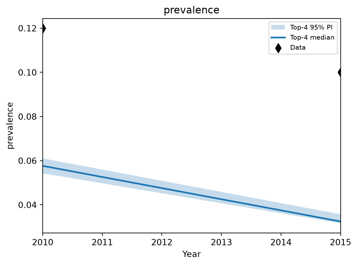
The default parameters are a point of departure, not a description of your setting. Calibration finds the values that best explain the data you have — and for cervical cancer that data is usually thin: a registry with counts by age band for one or two years, perhaps an HPV prevalence survey, perhaps a genotype distribution among a few hundred cases. The workflow is built around that, not around dense time series.
hpv.Calibration wraps Starsim’s calibration machinery, which uses Optuna to search the parameter space. You give it a sim, the parameters to vary, and the data.
Telling it what your data is
Targets go in as one table, with a float year index named t and column names that say what each column is:
Column form
Meaning
Where the model value comes from
all_hpv.<name>
One number per year
sim.results.all_hpv.<name> — for example all_hpv.asr_cancer_incidence
You can also pass a dictionary of data frames, or a list of long-format CSVs with columns year, name, [age, sex, genotype,] value.
Age-stratified columns configure the model for you: HPVsim reads the band labels ('0-30', '70+') for the bin edges and the index for the years, attaches a by_age analyzer with those settings, and extends sim.pars.stop past your last data year if the sim would have finished too early. Keeping analyzer bins and registry bins in sync by hand is a common source of quiet error, and this removes it.
Missing cells are allowed: NaN is skipped, so a registry reporting 2015 and 2019 but not the years between costs you nothing.
Choosing parameters and reading the mismatch
calib_pars is nested by scope, and each leaf is a list: [best guess, low, high, step], with step optional.
The scopes are the same ones described in Parameters. Flat dotted keys, and the older dict(low=..., high=..., guess=...) leaf form, are no longer accepted — both raise an error telling you which form to use.
Mismatch is a weighted sum over columns. Each column’s error is normalized by the largest observed value in it, so a cancer count in the thousands and a prevalence of 0.1 contribute comparably; weights={'all_hpv.prevalence': 2.0} then adjusts deliberately. Because normalization depends on the data you supplied, mismatch values are comparable within one calibration and meaningless between two.
Two defaults exist because of how rare cervical cancer is. reseed=False keeps the random seed fixed across trials — with reseeding, cancer counts move more with the seed than with the parameters, and the search converges on the luckiest seed rather than the best parameters. And Optuna trials are stored in an append-only journal file rather than SQLite, which deadlocks past about 32 concurrent workers.
Checking whether the fit is real
A single best-fitting trial tells you very little when the outcome is a handful of rare events. Look at the spread of the best trials instead: hpv.plot_calibration re-runs the top trials and draws the model’s range against your data, one panel per target. calib.df holds every trial’s mismatch and parameter values — a flat mismatch across a parameter’s full range means your data cannot identify it, so fix it to a literature value rather than let the search wander.
To inspect any output other than your targets, re-run the best trials with hpv.make_calib_sims(calib, n=50, extract_fn=...); without an extract_fn you get 50 full sims back, which is many gigabytes. Use calib.shrink() before committing a calibration to source control.
How to run a first calibration
Start deliberately small. A handful of trials on a small population tells you whether the plumbing works — that the data is read, the parameters move, and the mismatch responds. Only then scale up trials and population.
[I 2026-09-19 16:44:52,619] A new study created in Journal with name: hpvsim_calibration
<optuna.storages.journal._storage.JournalStorage object at 0x776a1d72fc10>
[I 2026-09-19 16:44:53,308] Trial 0 finished with value: 1.1170912322898707 and parameters: {'beta': 0.1, 'hpv16.cin_fn.k': 0.35}. Best is trial 0 with value: 1.1170912322898707.

[I 2026-09-19 16:44:53,327] Trial 1 finished with value: 1.1170912322898707 and parameters: {'beta': 0.1, 'hpv16.cin_fn.k': 0.35}. Best is trial 0 with value: 1.1170912322898707.

[I 2026-09-19 16:44:53,833] Trial 2 finished with value: 1.02317247291406 and parameters: {'beta': 0.2, 'hpv16.cin_fn.k': 0.4}. Best is trial 2 with value: 1.02317247291406.

[I 2026-09-19 16:44:53,852] Trial 3 finished with value: 1.13137546988825 and parameters: {'beta': 0.35, 'hpv16.cin_fn.k': 0.15}. Best is trial 2 with value: 1.02317247291406.

[I 2026-09-19 16:44:54,511] Trial 4 finished with value: 1.0911397735277812 and parameters: {'beta': 0.2, 'hpv16.cin_fn.k': 0.35}. Best is trial 2 with value: 1.02317247291406.

[I 2026-09-19 16:44:54,516] Trial 5 finished with value: 1.0768554893632731 and parameters: {'beta': 0.4, 'hpv16.cin_fn.k': 0.2}. Best is trial 2 with value: 1.02317247291406.
Six trials over two parameters is a plumbing test, not a calibration. For real work: fit the sexual network to behavioral data first, then transmission to prevalence, then progression to cancer, adding parameters only where the data can identify them. Expect several hundred to a few thousand trials, and run those on a machine you are not also using for anything else.
Coverage runs matter more than trial counts. Before spending compute, run 50 parameter sets drawn from your ranges and check that your data falls inside the resulting spread. If it does not, no number of trials will help — the model as configured cannot produce your data, and something structural (network, demographics, the target itself) needs attention first.