An analyzer watches a run and records something the standard results do not cover. It never changes what happens in the model. In this tutorial we use three of them: cancers in the age bands our data uses, how long HPV takes to become cancer, and the DALYs that burden represents. Then we write one of our own.
Cancers in your data’s age bands
Cancer registries typically report cases by five- or ten-year age bands. hpv.by_age records any age-stratified result at whatever bins and years you name.
Here we match the bands in nigeria_cancer_cases.csv, an age-stratified count of cervical cancer cases in Nigeria in 2020, collapsed to ten-year bands:
The first argument is the list of results you want by age. The choices are counts (n_infected, n_cin, n_cancerous, n_precin, hpv), annual event flows (cancers, cins), and prevalences (hpv_prevalence, cin_prevalence, cancer_prevalence, precin_prevalence).
Retrieve the analyzer from the finished run — not from the variable you created, which is a template the sim copied — and ask for a table:
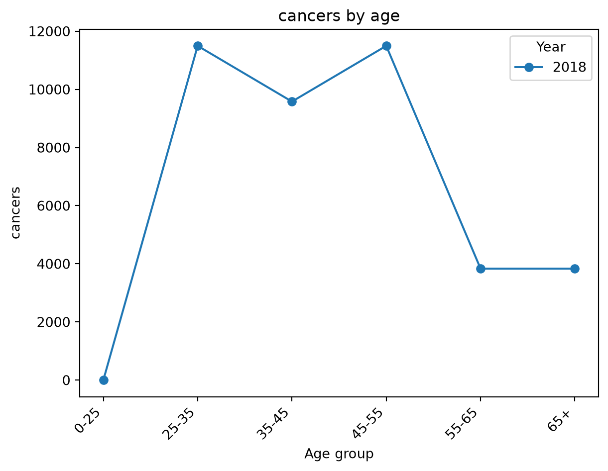
One row per year, one column per age band. Look at the individual rows: bands jump between zero and several thousand from one year to the next. At 2,000 agents a single calendar year holds only a handful of cancer events, each carrying a large population weight. Averaging over several years gives something you can actually compare against data:
Read the ratio column. The uncalibrated defaults overstate cancer counts, and the size of the discrepancy varies across age bands rather than being a constant factor — so this is not something you can fix by scaling the output. Part of the gap is real under-ascertainment in registry data; the rest is that the parameters have never been fitted to Nigeria. Closing it is what Tutorial 7 is about.
The same analyzer also recorded HPV prevalence by age:
Compare which band the peak falls in against prevalence surveys for your own setting. Most surveys put the peak in women in their early twenties. The age at which prevalence peaks is a second calibration target, and an informative one: it constrains the sexual-behavior parameters rather than the natural-history ones.
Each age band is also available as a timeseries of its own, named after the band:
fig = hpv.plot_by_age(by_age, 'cancers', years=[2018])print('Cancers in women 35-44, last four timesteps:', np.round(sim.results.by_age.cancers_35_45[-4:], 0))
Cancers in women 35-44, last four timesteps: [ 0. 0. 1916. 1916.]
How long does HPV take to cause cancer?
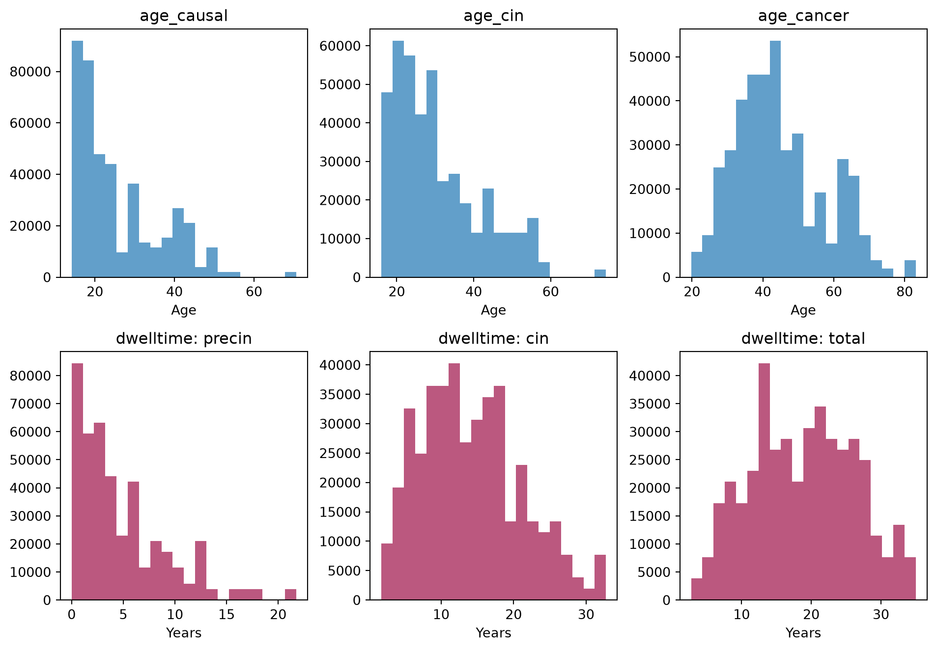
hpv.age_causal_infection traces every cancer back to the infection that caused it, and records how long each stage took:
history = sim.analyzers['age_causal_infection']w = history.weightsprint(f'Mean age at the infection that caused cancer: 'f'{np.average(history.age_causal, weights=w):.1f}')print(f'Mean age at precancerous lesion: 'f'{np.average(history.age_cin, weights=w):.1f}')print(f'Mean age at cancer: 'f'{np.average(history.age_cancer, weights=w):.1f}')for stage in ('precin', 'cin', 'total'):print(f' time in {stage:7s}: {np.average(history.dwelltime[stage], weights=w):.1f} years')
Mean age at the infection that caused cancer: 25.7
Mean age at precancerous lesion:              30.5
Mean age at cancer:                           44.6
  time in precin : 4.8 years
  time in cin    : 14.0 years
  time in total  : 18.8 years
The dwell times show where those years go. Most of the time between infection and cancer is spent as a precancerous lesion, and that long lesion stage is why screening works at all — it is the window in which a woman can be found and treated. It is also why a vaccination program takes decades to show up in cancer statistics.
fig = history.plot()
Turn cancers into DALYs
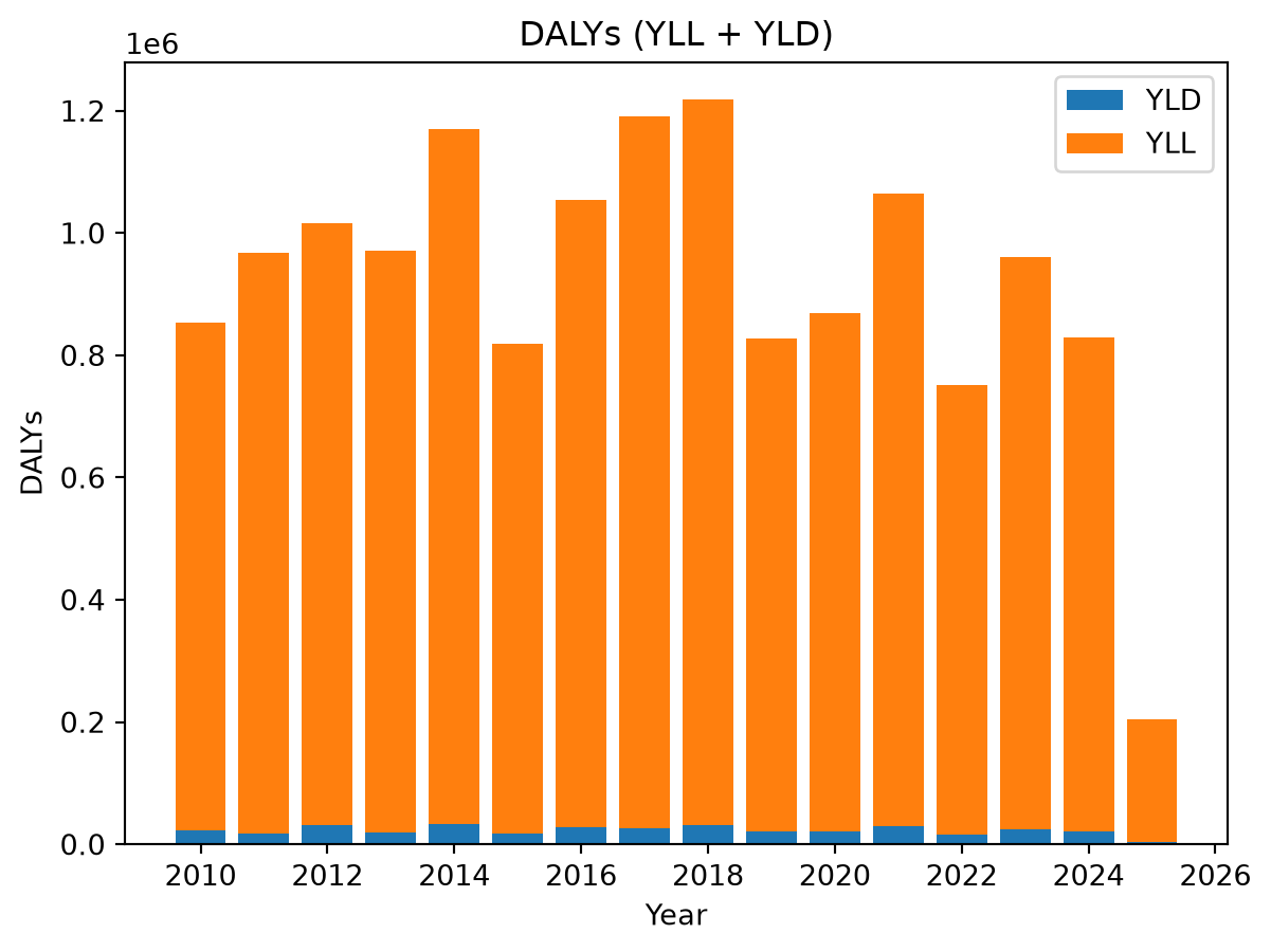
hpv.dalys converts cancer cases into years of life lost and years lived with disability, using GBD 2017 disability weights and a reference life expectancy of 84 years:
burden = sim.analyzers['dalys']i2020 = burden.years ==2020print(f'DALYs in 2020: {float(burden.dalys[i2020][0]):>10,.0f}')print(f' of which YLL: {float(burden.yll[i2020][0]):>9,.0f}')print(f' of which YLD: {float(burden.yld[i2020][0]):>9,.0f}')fig = burden.plot()
DALYs in 2020:    869,807
  of which YLL:   848,006
  of which YLD:    21,801
Almost all of the burden is years of life lost, not years lived with disability. Cervical cancer kills women in their forties and fifties, so each case costs decades of life. Pass life_expectancy= to use a national figure instead of the reference one.
Write your own
An analyzer is a class with two methods: init_results declares what it records, and step records it once per timestep. Here is one that answers a question a program manager would ask — how many women in the screening age range have never been screened?
import starsim as ssclass UnscreenedWomen(ss.Analyzer):"""Count women aged 30-49 who have never been screened."""def init_results(self):super().init_results()self.define_results( ss.Result('n_unscreened', dtype=float, scale=True, label='Women 30-49 never screened'), )def step(self): people =self.sim.people in_range = (people.alive & people.female& (people.age >=30) & (people.age <50)) screen =self.sim.interventions.get('screen')if screen isnotNone: in_range = in_range &~screen.screenedself.results.n_unscreened[self.ti] = people.scale_flows(in_range.uids)
scale=True on the result tells HPVsim this is a count of people, so it gets multiplied up to national scale like every other count. people.scale_flows handles the per-agent weighting that ms_agent_ratio introduces.
Never screened in 2014:   17,765,992
Never screened in 2020:    8,103,786
Never screened in 2030:    7,418,081
The number falls sharply once the program starts, then flattens as new women age into the range faster than the program reaches them. That flat line is the unmet need a real program has to plan for.