import numpy as np
import pandas as pd
import hpvsim as hpv

pd.read_csv('nigeria_cancer_types.csv')| year | name | genotype | value | |
|---|---|---|---|---|
| 0 | 2015 | cancerous_genotype_dist | 16 | 0.524 |
| 1 | 2015 | cancerous_genotype_dist | 18 | 0.145 |
| 2 | 2015 | cancerous_genotype_dist | ohr | 0.285 |
Tutorial 6 showed the uncalibrated model overstating cervical cancer counts in Nigeria, by an amount that varied across age bands. Calibration is how you fix that: you name the parameters you are willing to change, hand over your data, and let the model search for the values that reproduce it. In this tutorial we fit two parameters to Nigerian cancer data and look at the result.
The parameters that ship with HPVsim are generic, not a fit to any country. Calibration is a required step.
Three kinds of target, in the format cancer data usually arrives in:
year, name, age, sex, genotype, value.age column.genotype column and no age column.nigeria_cancer_cases.csv is the first kind and nigeria_cancer_types.csv is the third. Look at the second one before going further:
import numpy as np
import pandas as pd
import hpvsim as hpv
pd.read_csv('nigeria_cancer_types.csv')| year | name | genotype | value | |
|---|---|---|---|---|
| 0 | 2015 | cancerous_genotype_dist | 16 | 0.524 |
| 1 | 2015 | cancerous_genotype_dist | 18 | 0.145 |
| 2 | 2015 | cancerous_genotype_dist | ohr | 0.285 |
Its genotype column uses the names HPVsim knows: 16, 18, and ohr for the pooled other-high-risk group. Genotype labels in your own data will not necessarily match, and a label the model cannot resolve makes the whole calibration fail, so check them first. The names HPVsim accepts are in hpv.GENOTYPE_KEYS.
Now load both targets. Pass a list of file paths, DataFrames, or a mix:
targets = hpv.data.load_calib_data(['nigeria_cancer_cases.csv',
                                    'nigeria_cancer_types.csv'])
targets.T.head(6)| t | 2020.0 | 2015.0 |
|---|---|---|
| all_hpv.cancers.0-15 | 0.0 | NaN |
| all_hpv.cancers.15-20 | 25.0 | NaN |
| all_hpv.cancers.20-25 | 333.0 | NaN |
| all_hpv.cancers.25-30 | 858.0 | NaN |
| all_hpv.cancers.30-35 | 1231.0 | NaN |
| all_hpv.cancers.35-40 | 1534.0 | NaN |
The loader reshapes everything into one table: rows are years, and each column is one target value. Column names tell you where the model will look for the matching number — all_hpv.cancers.40-45 is pooled cancers in women aged 40 to 44, and by_genotype.cancerous_genotype_dist.hpv16 is HPV16’s share of cancers. Missing combinations are NaN and are skipped.
You do not need to add a hpv.by_age analyzer yourself. The calibration reads the age bands out of your data and attaches one that matches.
Group them by what they belong to, and give each one a list: [starting value, lowest, highest, step].
calib_pars = dict(
    beta = [0.25, 0.15, 0.35, 0.05],                                # Overall transmissibility
    hpv16 = dict(
        cancer_fn = dict(transform_prob=[2e-3, 1e-3, 4e-3, 5e-4]),  # HPV16 lesion-to-cancer rate
    ),
)
A bare key is a whole-sim parameter. A key nested under a genotype name (hpv16, hpv18, hi5, ohr) is that genotype’s parameter, nested as deeply as the parameter itself is. A key nested under network is a partnership parameter, and one under cross_immunity is a cross-protection parameter.
Note that the sim runs the three genotype groups the data reports, so every observed share maps onto exactly one modeled group. If you run genotypes your data does not distinguish, you have to decide how to split the observed share between them — and there is usually no defensible way to do it.
Two parameters is a small fit, chosen so this tutorial runs in seconds. beta sets how much cancer there is overall; transform_prob sets how readily HPV16 lesions turn cancerous, which shifts the age pattern.
def make_sim():
    """The sim the calibration will vary and re-run."""
    return hpv.Sim(
        location       = 'nigeria',
        genotypes      = [16, 18, 'ohr'],   # Exactly the groups the data reports
        n_agents       = 2000,
        start          = 1990,
        stop           = 2021,
        ms_agent_ratio = 25,
        rand_seed      = 0,
        verbose        = 0,
    )

calib = hpv.Calibration(
    make_sim(),
    calib_pars,
    data         = targets,
    total_trials = 4,      # Far too few; see below
    n_workers    = 2,
    verbose      = 0,
)
calib.calibrate()
print('Best fit:', calib.best_pars)
[I 2026-09-19 16:46:59,615] A new study created in Journal with name: hpvsim_calibration
Best fit: {'beta': 0.2, 'hpv16.cancer_fn.transform_prob': 0.001}Every trial runs the model once with a different combination of parameter values, scores how far the model is from your data, and reports the score as mismatch — smaller is better. The trials are ranked:
calib.df| index | mismatch | beta | hpv16.cancer_fn.transform_prob | |
|---|---|---|---|---|
| 0 | 0 | 16.334150 | 0.20 | 0.0010 |
| 2 | 2 | 23.947955 | 0.30 | 0.0020 |
| 1 | 1 | 24.782443 | 0.35 | 0.0035 |
| 3 | 3 | 37.895449 | 0.35 | 0.0030 |
fig = hpv.plot_calibration(calib, top_n=4)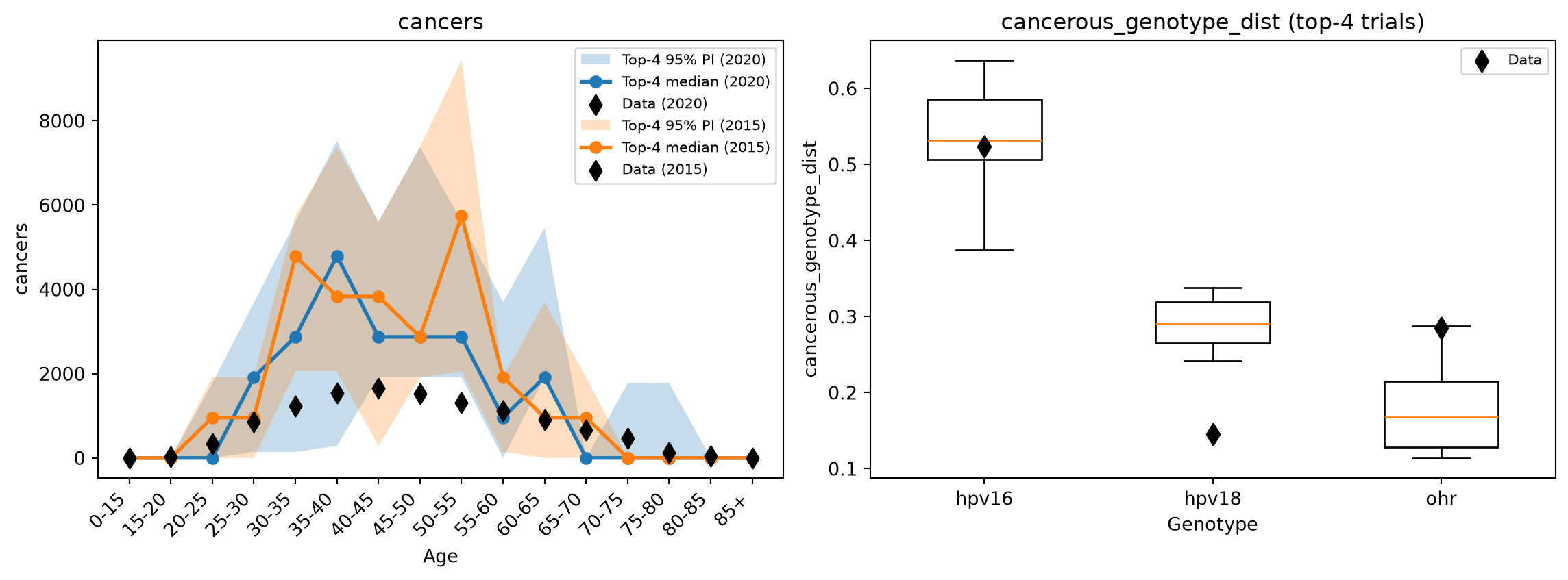
One panel per target. The age panel shows your data as points and the best trials as a band; the genotype panel shows the same as boxes against your observed shares.
Read the shape, not the score. A run that lands on the right total but the wrong age pattern will score similarly to one that is uniformly too low, and only the first is useful. If the band misses your points in the same direction across every age band, the parameters you opened up cannot reach your data — open different ones rather than running more trials.
This fit is a demonstration of the mechanics. A real calibration needs:
total_trials to at least a few hundred and n_workers to the number of cores you have. That belongs on a server, not a laptop.n_agents=2000 the model’s own noise is comparable to the differences between parameter sets, so the search partly fits noise. Raise n_agents until repeated runs of the same parameters agree closely.The random seed stays fixed across trials, because reseed=False is the default. This matters for HPV: cancer is rare, so if each trial also drew a new seed, the search would find the luckiest seed rather than the best parameters.
A finished calibration object is large. shrink() keeps only what you need to replot it or rebuild the best sims, which is small enough to commit alongside your analysis:
compact = calib.shrink()
compact.best_pars
{'beta': 0.2, 'hpv16.cancer_fn.transform_prob': 0.001}The calibration stores each trial’s score, not each trial’s full results. To look at anything else — a projection past your data years, an extra analyzer — re-run the best trials with hpv.make_calib_sims(calib, n=...) and read the sims it returns.