T1 - Getting started

In this tutorial we build a cervical cancer model for Nigeria, run it, read the cancer burden it produces, and measure how much of that burden HPV vaccination would prevent.

Install HPVsim

HPVsim is a Python package. Install it with:

pip install hpvsim

Then import it. The rest of this tutorial series uses hpv as the short name:

import hpvsim as hpv

The defaults are not fitted to your country

Read this before you read any number this model produces.

The parameters that ship with HPVsim are generic. They are not a fit to Nigeria or to anywhere else. A bare hpv.Sim(location=...) reproduces HPV prevalence reasonably well, but it overstates cervical cancer incidence — for Nigeria, by several times the rate the registries report.

So calibration is a required step, not an optional refinement. Everything in Tutorials 1 to 6 teaches you to drive the model and read its output; Tutorial 7 is where you make its output mean something about a real population. Until you have done that, treat the numbers below as a demonstration of the mechanics, and read differences between scenarios rather than absolute levels.

Set up a country model

Everything a run needs is a keyword argument to hpv.Sim. We collect them in a dictionary so later steps can reuse them:

pars = dict(
    location       = 'nigeria',                # Age structure, births and deaths for Nigeria
    genotypes      = [16, 18, 'hi5', 'ohr'],   # HPV16, HPV18, and two pooled high-risk groups
    n_agents       = 2000,                     # Number of simulated people
    start          = 1990,                     # First year
    stop            = 2070,                    # Last year
    ms_agent_ratio = 25,                       # Follow 25 cancer trajectories per lesion
    verbose        = 0,                        # Stay quiet while running
)

Three of these deserve a note.

location loads Nigeria’s age structure, birth rates and death rates from the UN World Population Prospects, and scales the results up to the real national population. Any country name in the WPP works, and the name is case-insensitive.

stop = 2070 looks far away, and it has to be. A woman infected today may develop cancer in twenty or thirty years, so a run that ends in 2040 cannot show you the effect of anything you start now.

ms_agent_ratio exists because cervical cancer is rare. In a 2,000-person run only a handful of women would ever reach cancer, so the yearly counts would jump around wildly. Setting ms_agent_ratio=25 follows 25 possible cancer trajectories for each woman who develops a precancerous lesion, and counts each one at a weight of 1/25. Cancer numbers steady down without simulating more people.

We leave the timestep at its default of a quarter of a year. HPVsim’s parameters are set up for that timestep, so change it only if you know why you are doing so.

Run it

sim = hpv.Sim(**pars)
sim.run()

Sim(n=2000; 1990—2070; demographics=births, deaths, agemigration; networks=sexualnetwork; diseases=hpv16, hpv18, hi5, ohr; connectors=crossimmunity, _exclusiveseeder; analyzers=all_hpv)

The run takes a few seconds. Now plot the two cancer outputs side by side — cumulative cases, and age-standardized incidence per 100,000 women per year, which is what cancer registries and GLOBOCAN report:

fig = sim.plot(['all_hpv_cum_cancers', 'all_hpv_asr_cancer_incidence'])

Figure(768x576)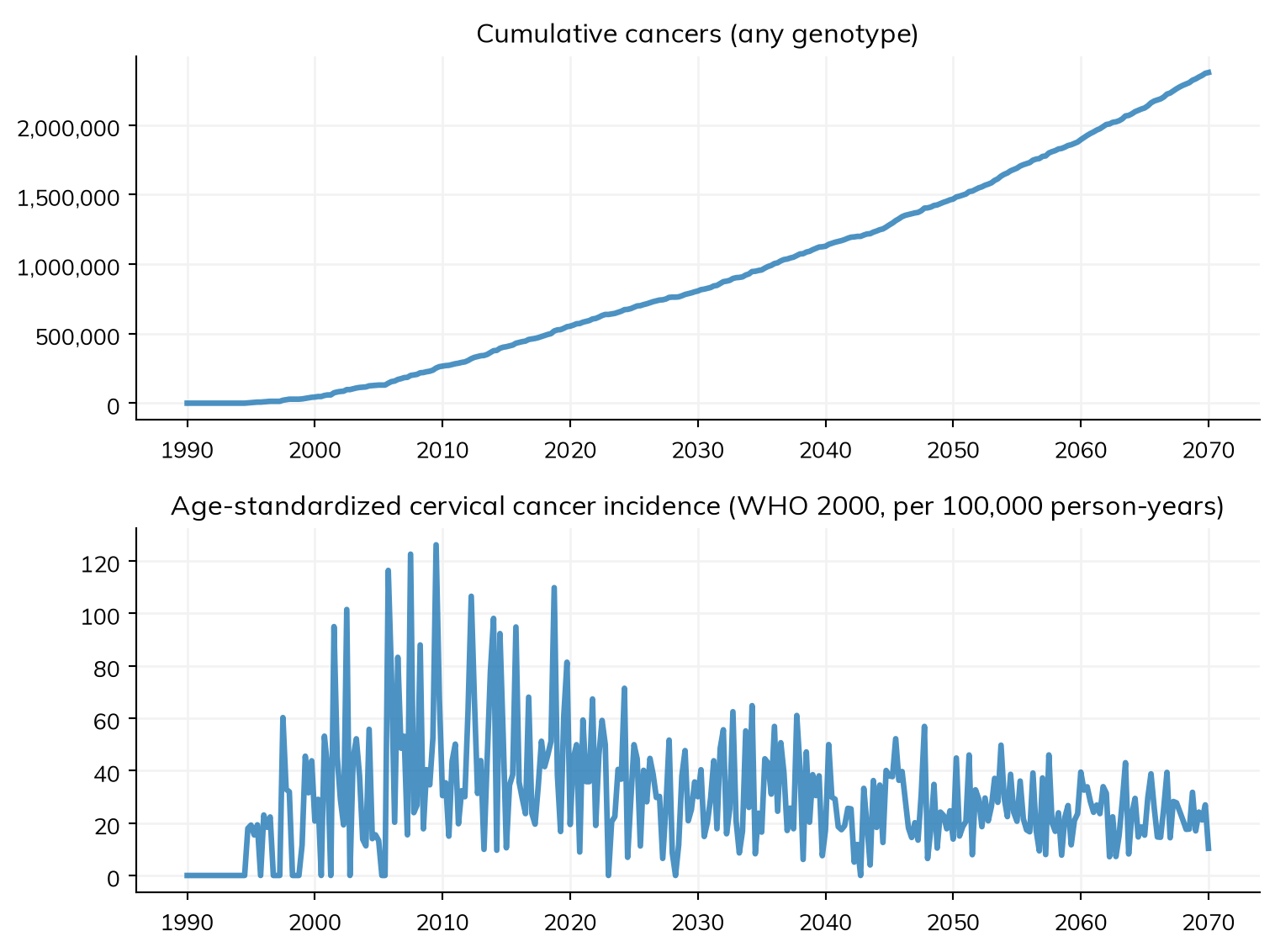

Compare the two panels. The cumulative curve rises smoothly. The incidence curve is jagged, and neighboring years disagree sharply. Both come from the same handful of simulated cancer events; the cumulative curve averages over all of them, while each year of the incidence curve rests on very few.

At n_agents=2000, read the cumulative panel. Treat any single year of the incidence curve as unreliable until you have checked it against several random seeds, which is what Tutorial 3 covers.

The final year is also incomplete: incidence for a calendar year is summed over the timesteps inside it, and the last year of a run has only one. Read the year before stop, never stop itself.

Find the numbers

Results are grouped by module. Each genotype has its own set, and all_hpv pools them:

years = sim.results.timevec.years                      # Calendar years
print('Cancers by 2070, all genotypes:',
      f'{float(sim.results.all_hpv.cum_cancers[-1]):,.0f}')
print('Cancers by 2070, HPV16 only:  ',
      f'{float(sim.results.hpv16.cum_cancers[-1]):,.0f}')
print('Cancers to 2020:              ',
      f'{float(sim.results.all_hpv.cum_cancers[years == 2020][0]):,.0f}')

Cancers by 2070, all genotypes: 2,377,929
Cancers by 2070, HPV16 only:   1,498,421
Cancers to 2020:               553,764

Compare HPV16’s share against genotyping studies for your own setting — it is one of the first things calibration should get right. To see the whole list of pooled results, use sim.results.all_hpv.keys().

Add a vaccination program

Now the question that motivates most HPVsim work: how much cancer does vaccinating girls prevent? We give the bivalent vaccine to 90% of girls aged 9 to 14 from 2015, and run that alongside the unchanged model:

import starsim as ss

vx = hpv.routine_vx(product='bivalent', prob=0.9, age_range=[9, 14],
                    start_year=2015)

s0 = hpv.Sim(**pars, label='No vaccination')
s1 = hpv.Sim(**pars, interventions=vx, label='Vaccination from 2015')

msim = ss.MultiSim([s0, s1])
msim.run(verbose=0)
fig = msim.plot('all_hpv_cum_cancers')

Figure(768x576)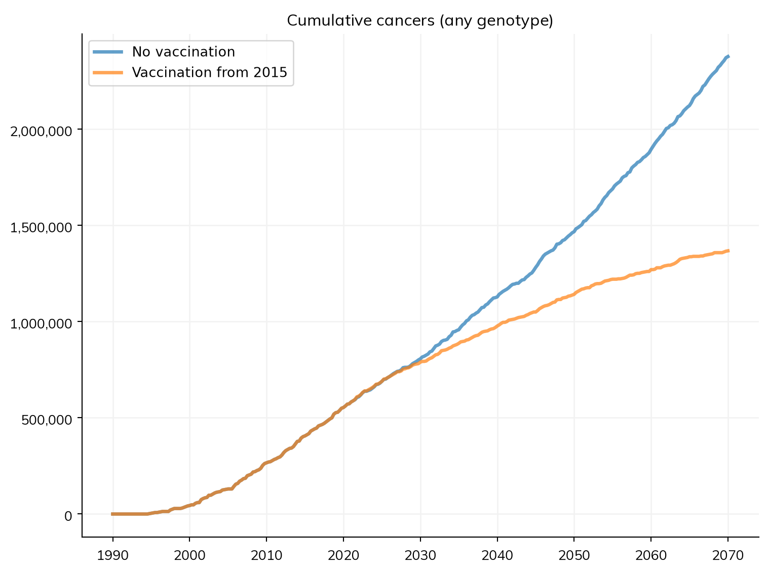

The two curves sit on top of each other for decades, then separate and keep diverging. That delay is real: girls vaccinated in 2015 do not reach the ages where cervical cancer occurs until the 2040s and beyond.

The headline number is cumulative cancers averted over the whole window:

baseline, vaccinated = msim.sims
c0 = float(baseline.results.all_hpv.cum_cancers[-1])
c1 = float(vaccinated.results.all_hpv.cum_cancers[-1])
print(f'Cancers 1990-2070, no vaccination:      {c0:>10,.0f}')
print(f'Cancers 1990-2070, with vaccination:    {c1:>10,.0f}')
print(f'Averted:                                {c0 - c1:>10,.0f}  ({(c0 - c1) / c0:.1%})')

Cancers 1990-2070, no vaccination:       2,377,929
Cancers 1990-2070, with vaccination:     1,368,124
Averted:                                 1,009,805  (42.5%)

Because the window starts in 1990, that percentage includes twenty-five years in which vaccination could not have changed anything, so it understates what the program does for girls alive today. When you report vaccination impact, always say which window you are reporting over.

Why not just quote one year?

It is tempting to pick a year and report the ratio between the two runs. Look at what happens if you do:

yrs = baseline.results.timevec.years
a0 = baseline.results.all_hpv.asr_cancer_incidence
a1 = vaccinated.results.all_hpv.asr_cancer_incidence
print(' year   no vaccine   vaccinated   ratio')
ratios = []
for y in (2020, 2030, 2040, 2045, 2050, 2060):
    v0 = float(a0[yrs == y][0])
    v1 = float(a1[yrs == y][0])
    ratio = v1 / v0 if v0 else float('nan')
    ratios.append(ratio)
    print(f' {y}     {v0:7.1f}      {v1:7.1f}     {ratio:5.2f}')
print(f'\nSpread across those years: {min(ratios):.2f} to {max(ratios):.2f}')

 year   no vaccine   vaccinated   ratio
 2020        19.4         19.4      1.00
 2030        30.0         36.9      1.23
 2040        17.4         35.7      2.06
 2045        38.0          0.0      0.00
 2050        13.9          9.5      0.68
 2060        39.4         26.2      0.66

Spread across those years: 0.00 to 2.06

Look at the spread on the last line. Neighboring years can disagree by a wide margin, and a year can even come out above 1 — saying vaccination made things worse — purely because that year happened to hold a cluster of cancer events in one run and not the other.

This is why impact should be reported as cumulative burden over a stated window, or as a median across several random seeds. A single year at this population size can point either way.

Where to next

Tutorial 2 covers plotting and saving, Tutorial 3 covers running many simulations at once and putting uncertainty bands on a result, and Tutorial 5 covers screening and treatment programs. Tutorial 7 covers calibration, which is what turns any of this into a statement about a real population.